我一直想做这个事情来着,现在终于有时间闲下来写一写了。
这个东西的目的是让自己对Transformer有一个更深入的理解,同时也能让一些人不需要装torch或者是llama.cpp这些相关依赖,就能大概运行起来LLaMA,甚至是训练,不过CPU实在是太慢了。
我不打算实现自动求导,而选择手动对每一部分计算梯度,直接写死在代码里。我有点后悔了,手算梯度实在是太痛苦了。
Linear Layer
首先最开始,我们来实现标准的线性层。
对于一个线性层
我们可以很容易的计算出梯度
写成矩阵形式就是
但是实际上在使用的时候,我们往往会把线性层堆叠起来构成深度的网络,所以在算梯度时候需要考虑下游的梯度。
这里我们假设输出$y$之后的下游部分为$f(y)$,那么我们可以用链式法则计算出参数的梯度:
同时,传给上游的梯度为:
用代码简单实现一下:
def backward(self, grad_output):
    x = self.x
    self.grad_weights = grad_output.T @ x
    self.grad_bias = np.sum(grad_output, axis=0)
    return grad_output @ self.weights
Activation Function
激活函数有很多,比如常见的ReLU:
class ReLU(Module):
    def __init__(self):
        super().__init__("ReLU")

    def forward(self, x):
        self.x = x
        return np.maximum(x, 0)

    def backward(self, grad_output):
        index = self.x > 0
        grad_input = grad_output * index
        return grad_input
这里面比较复杂的是Softmax,这里参考了这篇文章。
# Softmax
def backward(self, grad_output):
    softmax_dim = self.softmax.shape[-1]

    identity_shape = (self.softmax.shape[0],) + (1,) * self.softmax.ndim # (batch_size, 1, 1, ..., 1)
    identity = np.identity(softmax_dim, dtype=self.x.dtype)
    identity = np.tile(identity, identity_shape)

    first_term = self.softmax[..., np.newaxis] * identity

    expanded = self.softmax[..., np.newaxis]
    second_term = expanded @ self.softmax[..., np.newaxis, :]

    J = first_term - second_term

    grad_input = grad_output[..., np.newaxis, :] @ J
    return grad_input.reshape(self.x.shape)
但是一般我们也不会直接用Softmax,而是在CrossEntropyLoss中使用,这时候一般会把(\log)和和Softmax合并成一个函数,此时梯度会简单很多:
# LogSoftmax
def backward(self, grad_output):
    grad_input = grad_output - self.softmax * np.sum(grad_output, axis=self.axis, keepdims=True)
    return grad_input
Loss Function
我只实现了MSELoss和CrossEntropyLoss,毕竟不是在写完整的框架,这两个肯定是够用了。
MSELoss就很简单了:
def loss(self, y, label):
    y = np.asarray(y)
    label = np.asarray(label)
    mse_loss = (y - label) ** 2

    if self.reduction == 'mean':
        return np.mean(mse_loss)
    elif self.reduction == 'sum':
        return np.sum(mse_loss)
    else:
        raise ValueError(f"reduction {self.reduction} is not supported")

def grad(self, y, label):
    num_instances = np.prod(y.shape)
    if self.reduction == 'sum':
        num_instances = 1

    y = np.asarray(y)
    label = np.asarray(label)

    return 2 * (y - label) / num_instances
CrossEntropyLoss就不多赘述了,都是类似的东西。
Training
到这里,我们现有的组件(线性层,激活函数,损失函数)就已经足够训练一个简单的网络了。
拍脑袋想一个最简单的任务
x: [1, 2, 3, 4, 5]
y: [x[0] + x[2] + x[4], max(x[1], x[3])]
然后构造一个只有两层的MLP,应该是足够处理这个任务了
xdim = 5
ydim = 2

model = layers.Sequential(
    layers.Linear(xdim, 32),
    layers.ReLU(),
    layers.Linear(32, ydim)
)
接着就可以愉快地开始训练了
loss_fn = MSELoss()
learning_rate = 0.01

for epoch in range(100):
    indices = np.random.permutation(data_size)
    average_loss = 0.0
    for i in range(data_size // batch_size):
        batch_indices = indices[i*batch_size:(i+1)*batch_size]
        y_pred = model.forward(x[batch_indices])
        loss, grad = loss_fn(y_pred, y[batch_indices])
        model.backward(grad)
        model.step(learning_rate)
        average_loss += loss
        if (i + 1) % 10 == 0:
            print(f"Epoch {epoch+1}, Iteration {i+1}, Loss {average_loss / 50}")
            average_loss = 0.0
可以看到loss是在正常下降的
Epoch 98, Iteration 10, Loss 0.0021909273733704414
Epoch 98, Iteration 20, Loss 0.0021747556001297007
Epoch 98, Iteration 30, Loss 0.002415027525976499
Epoch 99, Iteration 10, Loss 0.002033462687265005
Epoch 99, Iteration 20, Loss 0.0024055140738835513
Epoch 99, Iteration 30, Loss 0.0023627760709594857
Epoch 100, Iteration 10, Loss 0.0021904293227183475
Epoch 100, Iteration 20, Loss 0.002405154366941388
Epoch 100, Iteration 30, Loss 0.002122699694332097
最后看一眼训练结果
Input values:
 [[0.1 0.2 0.3 0.4 0.5]
 [0.2 0.4 0.6 0.8 1.0 ]]

True values:
 [[0.9 0.4]
 [1.8 0.8]]

Predicted values:
 [[0.92035226 0.38735358]
 [1.80075877 0.76771189]]
看起来没什么问题,到这里,我们成功手写了几层神经网络,并且支持SGD的训练了。
Transformer
现在我们开始正式来实现Transformer的各个部分。
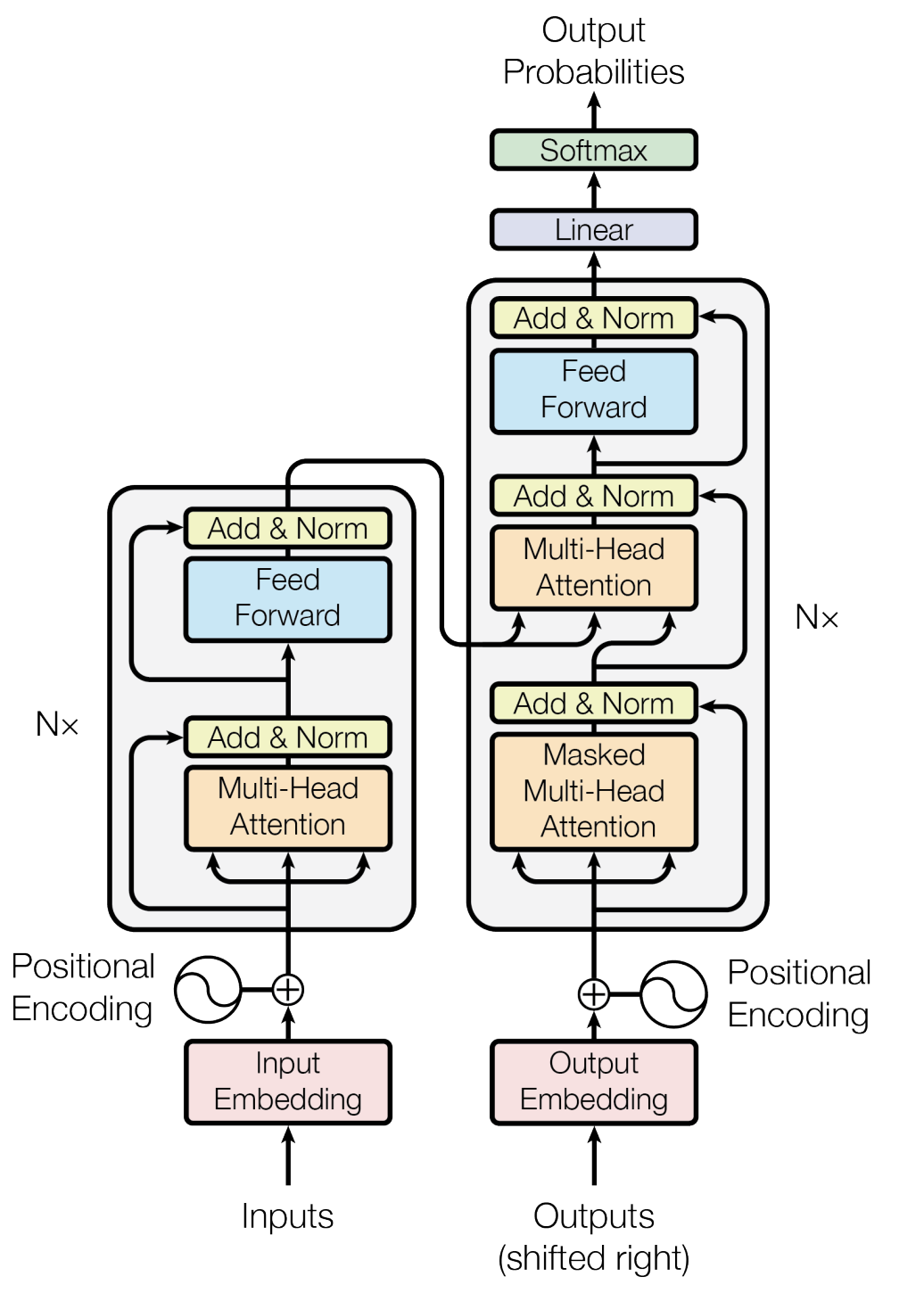
整体来看,需要实现四个部分:Embedding / Encoding,Multi-Head Attention,Feed Forward,Layer Normalization。
Embedding / Encoding
Embedding某种意义上就是一个特殊的线性层,只需要把输入的index转化为one-hot向量。这里我就直接按照矩阵乘法的方式来写了,其实应该需要take index来操作,矩阵乘法会占用大量的内存。
Encoding主要是Positional Encoding,原始论文里用的是sine和cosine函数:
论文也提到说可以用learned positional embedding,结果差不多。BERT里用的是后者,所以无法接受比训练时候更长的序列。
Multi-Head Attention
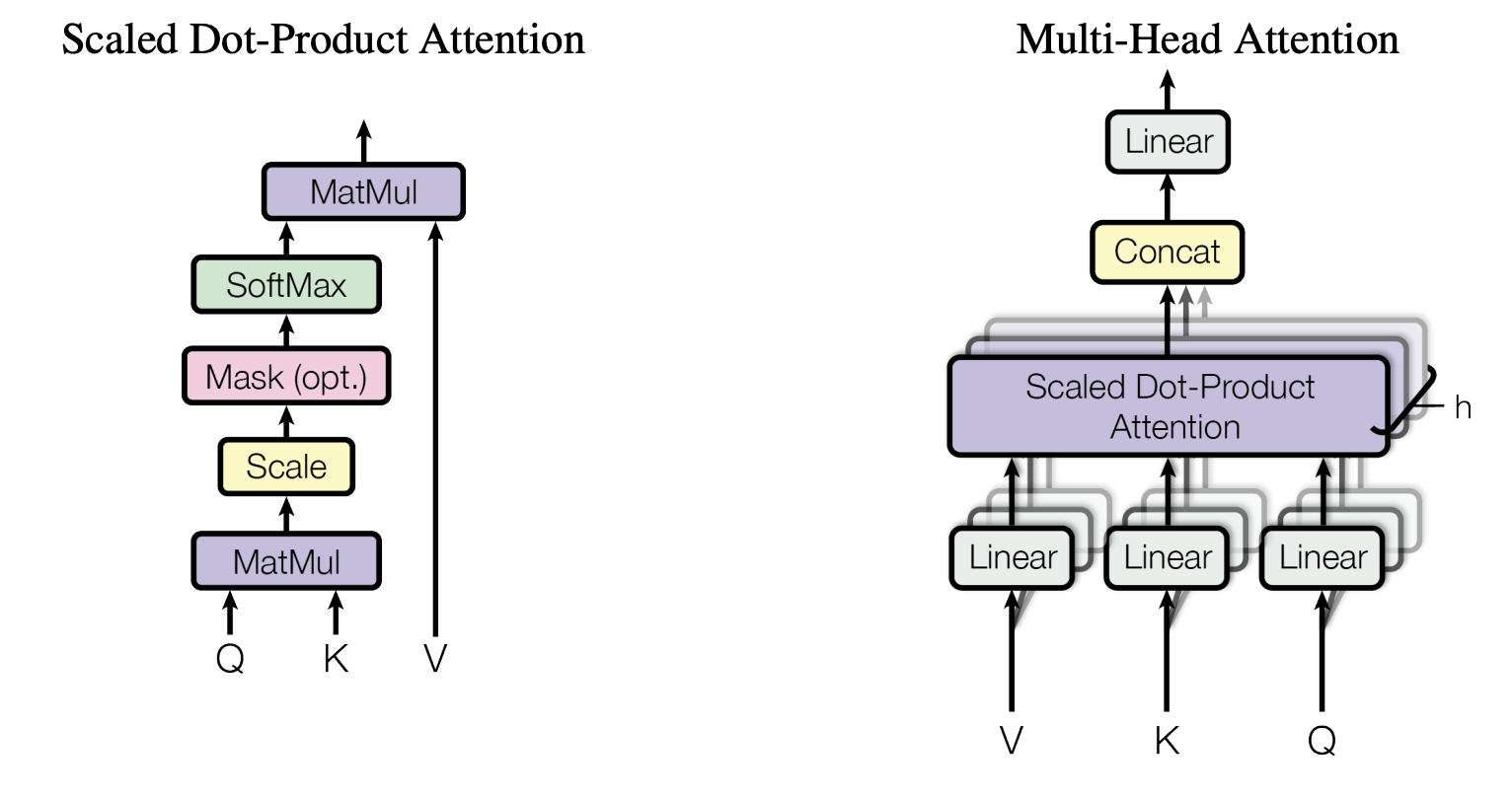
Multi-head Attention实在是太经典了,所以不多介绍了:
对于Scaled Dot-Product Attention,本质上就是矩阵乘法和Softmax,所以梯度计算很容易,配合上之前实现过的Softmax就行
def backward(self, grad_output):
    grad_v = self.attn.transpose(0, 1, 3, 2) @ grad_output

    grad_output = grad_output @ self.v.transpose(0, 1, 3, 2)
    grad_output = self.softmax.backward(grad_output)

    if self.mask is not None:
        grad_output = np.where(self.mask, grad_output, 0)

    grad_output = grad_output / np.sqrt(d_model)
    grad_q = grad_output @ self.k
    grad_k = grad_output.transpose(0, 1, 3, 2) @ self.q

    return grad_q, grad_k, grad_v
有了Scaled Dot-Product Attention,Multi-Head Attention的backward只需要按照链式法则调用Attention和四个线性层的backward就行了
def backward(self, grad_output):
    grad_output = self.W_o.backward(grad_output)

    batch_size, seq_len, _ = grad_output.shape
    grad_output = grad_output.reshape(batch_size, seq_len, self.num_heads, self.d).transpose(0, 2, 1, 3)

    grad_q, grad_k, grad_v = self.attention.backward(grad_output)

    grad_q = grad_q.transpose(0, 2, 1, 3).reshape(batch_size, seq_len, self.d_model)
    grad_k = grad_k.transpose(0, 2, 1, 3).reshape(batch_size, seq_len, self.d_model)
    grad_v = grad_v.transpose(0, 2, 1, 3).reshape(batch_size, seq_len, self.d_model)

    grad_q = self.W_q.backward(grad_q)
    grad_k = self.W_k.backward(grad_k)
    grad_v = self.W_v.backward(grad_v)

    return grad_q, grad_k, grad_v
只要注意一下维度变化,多个head直接concat起来,所以需要一直reshape和transpose。
Feed Forward
这个更简单,两个线性层加上一个ReLU。
def forward(self, x, train=True):
    # x: (batch_size, seq_len, d_model)
    self.x = x
    x = self.linear1.forward(x)
    x = self.activation.forward(x)
    x = self.dropout.forward(x, train)
    x = self.linear2.forward(x)
    return x

def backward(self, grad_output):
    grad_output = self.linear2.backward(grad_output)
    grad_output = self.activation.backward(grad_output)
    grad_output = self.dropout.backward(grad_output)
    grad_output = self.linear1.backward(grad_output)
    return grad_output
Layer Normalization
Layer Normalization是最难写的部分,forward相对来说简单一些,只是做了一个均值和方差下的归一化,再用一组参数放缩和平移。
backward就比较复杂了,找了几个资料但是算出来的梯度和PyTorch对拍之后都有出入,最后没办法,还是得自己硬算。
对于参数$\gamma$和$\beta$的梯度,会比较简单
接着来推导一下对于$x$的梯度,翻出了当年统计机器学习课的作业。感叹一下我那时候是真能暴力推导
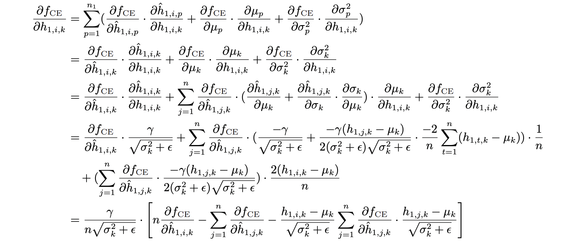
最后化简一下,剩下的形式是这样:
grad_norm = grad_output * self.gamma
grad_input = grad_norm \
 - grad_norm.mean(self.axis, keepdims=True) \
 - self.x_hat * (grad_norm * self.x_hat).mean(self.axis, keepdims=True)
grad_input *= self.std_inv
Encoder
现在,我们把这些部分组合堆叠起来,就可以得到一个完整的Transformer Encoder了。
# Encoder Layer
def forward(self, x, mask=None, train=False):
    x_ = self.multi_head_attention.forward(x, x, x, mask)
    x_ = self.dropout1.forward(x_, train)

    x = x + x_
    x = self.layer_norm1.forward(x)

    x_ = self.feed_forward.forward(x, train)
    x_ = self.dropout2.forward(x_, train)

    x = x + x_
    x = self.layer_norm2.forward(x)

    return x
BERT
现在让我们拿写好的东西,导入预训练好的BERT参数,看看能不能正常工作。
首先得看一下BERT里面的结构,我这里选用了一个较小一些的模型BERT-Tiny,只有两层encoder,每层有两个attention head,hidden size是128。
在Transformer Encoder之前,有标准的三种embedding,以及一个LayerNorm层(顺便这里还有一个Dropout)
bert.embeddings.word_embeddings.weight ([30522, 128])
bert.embeddings.position_embeddings.weight ([512, 128])
bert.embeddings.token_type_embeddings.weight ([2, 128])
bert.embeddings.LayerNorm.weight ([128])
bert.embeddings.LayerNorm.bias ([128])
然后是两个Encoder Layer
# attention
bert.encoder.layer.0.attention.self.query.weight ([128, 128])
bert.encoder.layer.0.attention.self.query.bias ([128])
bert.encoder.layer.0.attention.self.key.weight ([128, 128])
bert.encoder.layer.0.attention.self.key.bias ([128])
bert.encoder.layer.0.attention.self.value.weight ([128, 128])
bert.encoder.layer.0.attention.self.value.bias ([128])
bert.encoder.layer.0.attention.output.dense.weight ([128, 128])
bert.encoder.layer.0.attention.output.dense.bias ([128])
bert.encoder.layer.0.attention.output.LayerNorm.weight ([128])
bert.encoder.layer.0.attention.output.LayerNorm.bias ([128])

# feed forward
bert.encoder.layer.0.intermediate.dense.weight ([512, 128])
bert.encoder.layer.0.intermediate.dense.bias ([512])
bert.encoder.layer.0.output.dense.weight ([128, 512])
bert.encoder.layer.0.output.dense.bias ([128])
bert.encoder.layer.0.output.LayerNorm.weight ([128])
bert.encoder.layer.0.output.LayerNorm.bias ([128])
最后是一个prediction head
cls.predictions.bias ([30522])
cls.predictions.transform.dense.weight ([128, 128])
cls.predictions.transform.dense.bias ([128])
cls.predictions.transform.LayerNorm.weight ([128])
cls.predictions.transform.LayerNorm.bias ([128])
cls.predictions.decoder.weight ([30522, 128])
cls.predictions.decoder.bias ([30522])
看了下transformers的源码,这里的decoder.bias和bias是一样的。decoder的weights是与word_embeddings的weights保持一致的。所以本质上,这里就是对输出的embedding和word embeddings做了内积,然后加上了bias(没有bias的话其实是一个检索的过程)
Suffoquer's Blog
作诗中...